A Short History of Neural Synthesis
Introduction
22 May 2020
Dr Christopher Melen is PRiSM’s Research Software Engineer, designing and developing the tech that underpins our research and collaborations. In this first instalment on AI and music, Chris introduces neural synthesis, an exciting technique that features in the artistic work of the PRiSM team.
Neural synthesis is attracting widespread interest at this important time for AI and music – and is a key concept in PRiSM’s exploration of what it means for music to be co-created by human and computer.

Dr Christopher Melen
A Short History of Neural Synthesis
By Christopher Melen
The past few years have witnessed accelerated growth in interest in Machine Learning (ML) and Artificial Intelligence (AI) across many disciplines and sectors. One important enabling factor has been the emergence of software during this period, such as Google’s TensorFlow, and FaceBook’s PyTorch. This has made ML/AI more accessible to non-specialist users. The ubiquity of the Python programming language also cannot be ignored as a factor in this rapid development, given its approachability and relative ease of use, compared to languages such as C++. The recent ML/AI boom has led to a renewed interest in the use of computer-based tools and techniques in the creative disciplines, perhaps nowhere more prominently than in music.
Here, we focus on an area of research that has recently generated a lot of interest, that of ‘neural synthesis’ – sound generation based on Artificial Neural Networks. This article will provide an introduction to the topic, and give a brief overview of the solutions currently available in this area.
Artificial Neural Networks
To what do we owe the current AI boom? The birth of the web coincided with the start of the so-called ‘AI Winter’ which saw the first major wave of AI research come to a halt after a decade of hype, and eventual failure to live up to expectations. From this trough of the early 90s, enthusiasm for AI began to rekindle in the early years of the present century. Growth in interest from that time has been fuelled in part by the inevitable increase in computational capacity over time, the growth of the Cloud, and the greatly increased accessibility of hardware components such as GPUs. This steady growth has accelerated over the past decade due to the emergence of software solutions that have made Neural Networks more accessible and easier to program. Indeed, software ML platforms such as TensorFlow and PyTorch might be compared to the so-called ‘killer apps’ (graphical web browsers like Netscape, and web-based email), which led to the exponential growth of the Web in the mid-90s.
A Neural Network, or neural net, is a system made up of artificial neurons, input-output units modelled closely on the operations of cells in biological systems such as the brain. The earliest such networks date from the late 1950s, and were developed on specialised systems in research labs.
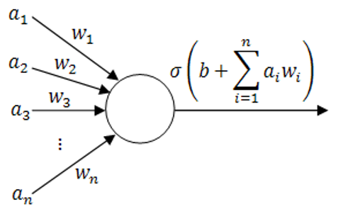
Figure 1: The Perceptron, the simplest type of neural network
Neural nets are typically built from several layers, each made up of one or more neurons. An input and output layer may together frame several internal or ‘hidden’ layers, with a single such layer consisting of several hundred or perhaps even thousands of cells. Artificial neurons themselves are, however, typically very simple structures, essentially input-output systems, to which random weights and biases are added. Figure 1 shows the perceptron, the simplest form of neural network, consisting of a single unit or neuron. Here we can see four separate inputs (an), each multiplied by a weight (wn). A bias unit value (b) is added to the sum of these and the result multiplied at the output by an activation function (s), whose value determines whether the neuron ‘fires’ or not.
In order for a neural network to learn it must be trained, which involves repeatedly exposing the network to a set of training data, a laborious process may take several hours, or even days, depending on the size and complexity of the input data. Over multiple ‘epochs’ or complete passes through the dataset, the weights and biases within each layer of the network are automatically adjusted and tuned.
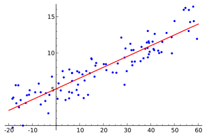
Figure 2: Linear regression, showing a set of random data points and the line of best fit (image courtesy of Wikipedia).
Historically, the process of training neural networks has a precursor in the mathematical concept of linear regression, which involves finding a ‘line of best fit’ for a set of data points. In both instances the degree of ‘fitness’ is measured using a loss function, which returns the error between the current training step and the dataset.
Our loss function should be lower at the end of training than at the beginning, a process known as minimizing the loss.
Once our network has been trained the resulting ‘model’ can be saved to persistent storage, and used to generate new output based on the learned source material.
Using TensorFlow, for example, it can take a matter of minutes to set up a network that can be trained on the complete Shakespeare Sonnets, and then used to generate passable imitations of The Bard’s work (the following excerpt is abridged from the TensorFlow site, licensed under Creative Commons Attribution 4.0 License):
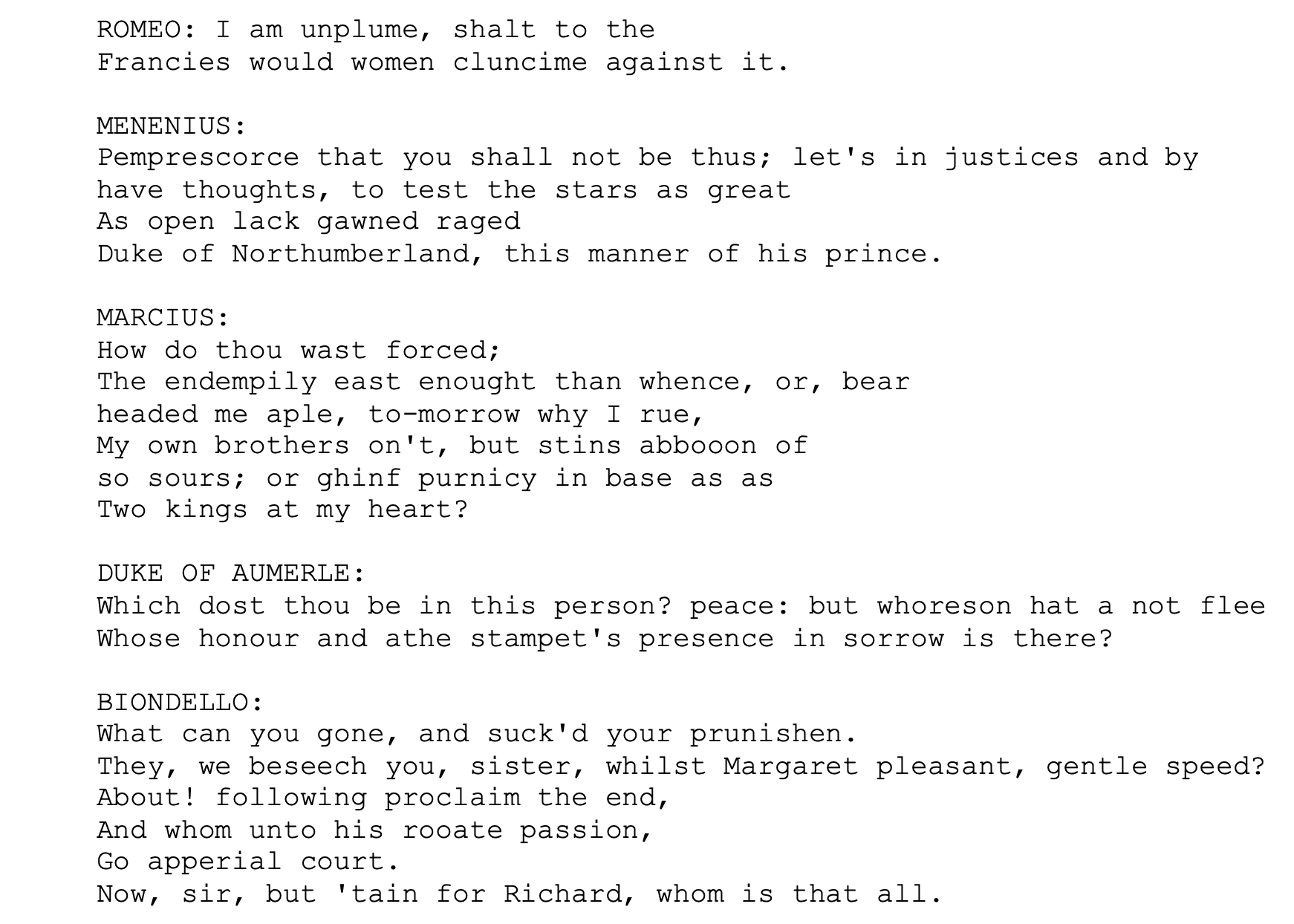
Well, if not imitations, perhaps, then… at least interesting variations. Note that the above is output generated after only a few epochs, and that greater accuracy can be achieved from further training, over many epochs.
Given the success shown by neural networks in modelling text, we might reasonably expect the same processes could, at least in principle, be brought to bear on other kinds of semantic sequences, for example music. It is important to recognise here the existence of two domains, one being audio signals, the other the symbolic representation of such signals, in forms such as written text or the musical score. Several attempts have been made at modelling the latter, for example OpenAi’s MuseNet, which processes and generates MIDI files. We will concentrate here on a different and arguably more interesting type of neural generative model, one which, rather than symbolic data, takes in raw audio signals, generating new audio signals at the other end. A number of such ‘end-to-end’ systems exist, the two most widely publicised of which are WaveNet and SampleRNN.
WaveNet
WaveNet, a system developed by the DeepMind project (supported by Google since 2014), uses neural networks to generate new audio from datasets of raw audio samples (see the 2016 article Wavenet: A Generative Model for Raw Audio). It was originally developed within the context of text-to-speech synthesis (TSS), but has also been taken up as a creative tool by musicians and composers (for example PRiSM’s own Sam Salem). WaveNet utilises a specific class of net, the Convolutional Neural Network (CNN or ConvNet), familiar from the domains of image processing and computer vision, where they have achieved great success in tasks such as image classification and feature detection. The basic operation of a CNN involves the incremental application of one or more filters across the 2-dimensional surface of an input image. Through a process of multiplication and summation these filters (or ‘kernels’) are able to summarize the pixel content of different portions of the image at a time. See a more detailed explanation here. For audio generation, being sequence-based, the dimensionality is reduced from 2 to the single dimension of time, but the basic principle and operation remains the same.
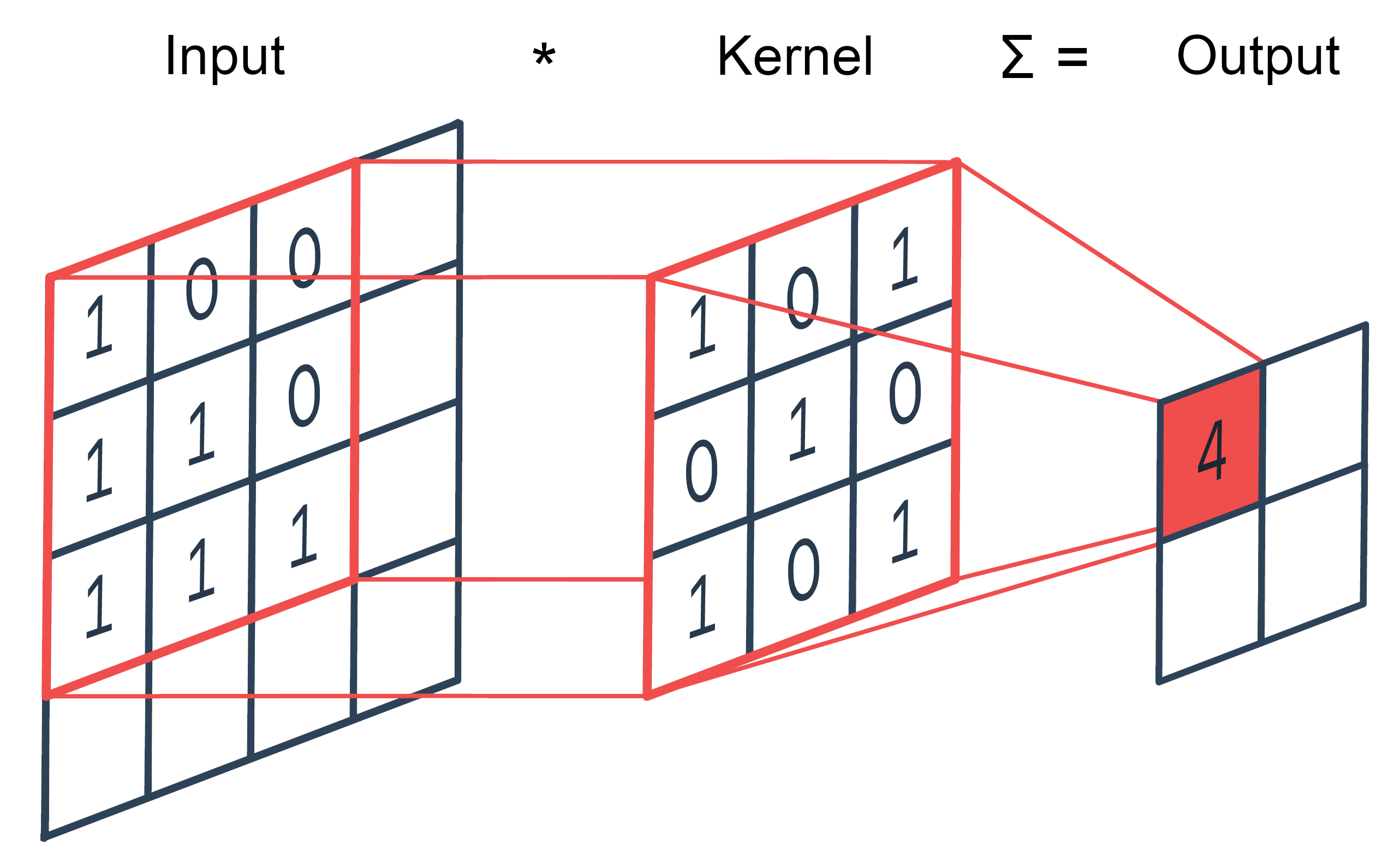
Figure 3: 2D Convolution. Each cell in the input matrix is first multiplied with the corresponding cell in the kernel. These new values are then summed, with the result representing a single cell in the output matrix. The whole process is repeated with the kernel shifted to the right by one or more steps, until the entire input matrix has been consumed.
WaveNet’s generative model is composed of multiple convolution layers, which combine to produce a probability distribution for the next sample, conditional on all previous samples. WaveNet uses a modified form of convolution involving a process called dilation (sometimes called ‘convolution with holes’), in which the outputs of successive hidden layers are ‘pruned’, with some outputs omitted as inputs to the next layer. As shown in Figure 4 below, at each new layer the input from the previous layer is dilated, the exponential increase in these dilations enabling the system to quickly expand to thousands of timesteps.
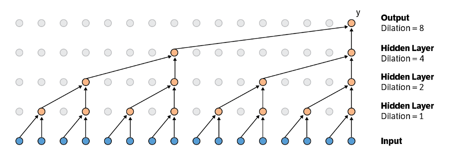
Figure 4: WaveNet architecture.
WaveNet has proven very successful at producing high quality audio output, particularly for speech synthesis where it represents a vast improvement on earlier efforts in this area (which typically involved concatenating many small samples from pre-existing audio, resulting in a ‘robotic’-sounding output). It is currently being used by Google in its Google Assistant product and elsewhere. Despite notable competitors, WaveNet remains the most popular model for neural audio generation in use today (a TensorFlow implementation can be found here). However, the conditional nature of the architecture, where each generated sample depends on ones from all previous steps, has a major performance impact. Since the network is essentially a binary tree, its overall computational cost is O(2^L), which makes the system impractical for large values of L.
Some audio examples generated using WaveNet can be found in Google’s text-to-speech documentation here, and also embedded in the original DeepMind blog post on the WaveNet architecture.
WaveNet has particularly impressive results in speech synthesis, where a discrete focus is a net positive. WaveNet has arguably had less success in modelling musical structure beyond a few seconds, which is not to say it is incapable of producing extended music sequences, but rather that their structural coherence tends to diminish as the time scales increase.
SampleRNN
Like WaveNet, SampleRNN directly processes raw audio samples, but differs in the type of neural net it uses. Whereas WaveNet is based on convolution networks, SampleRNN utilises a type of neural net known as Recurrent Neural Network, or RNN. Such networks were developed to process sequential data, such as time series, or anything that can be modelled in a sequential fashion such as text, and indeed audio data such as speech or music. Unlike simple ‘feed forward’ networks like the perceptron, RNNs retain a kind of internal ‘memory’ of their previous states (hence the label ‘recurrent’).
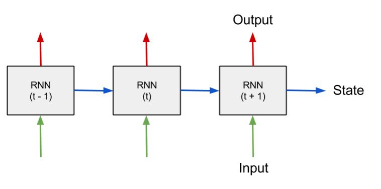
Figure 5: Recurrent Neural Network (RNN).
In Figure 5 we can see the basic RNN structure, ‘unrolled’ over several time steps, from t-1 to t+1. The output state from a unit at one step is fed in as the input state to the next. Note that this unrolled structure is here purely diagrammatic, since a typical RNN will actually consist of a single unit which iterates over the time steps in a loop, feeding its own output back into itself at each step. As well as ‘remembering’ these networks are also able to ‘forget’, with states beyond a certain configurable time limit being erased from history.
Like WaveNet the output of the SampleRNN model represents a probability distribution, from which the next sample can be predicted. As we noted when discussing WaveNet, one of the major problems in modelling audio signals is one of scale: structures within a signal often exist on multiple scales simultaneously, with samples having semantic relationships with both neighbouring samples and ones separated by many timesteps. A related issue is the discrepancy between the dimensionality of the raw audio input signal and this sample-by-sample output. With even a low sample rate of 16kHz we will typically need to produce many thousands of samples before any recognisable or useful output is produced. Modelling long-term dependencies in the input dataset is therefore inherently problematic.
To address these issues SampleRNN adopts a hierarchical architecture, consisting of separate recurrent networks layered on top of each other in tiers, with each tier having a wider temporal resolution than the one immediately below it. Sample frames of a fixed size are consumed at each tier, with the lowest tier resolving at the level of individual samples (the lowest tier is in fact not a RNN but rather a Multi-Layer Perceptron or MLP, a simple feed-forward network). Each tier except for the highest, is also conditioned by the output of the tier immediately above.
The SampleRNN architecture was publicly introduced in the paper SampleRNN: An Unconditional End-to-End Neural Audio Generation Model, presented at ICLR in 2017. The authors released an implementation shortly afterwards, made available on GitHub. The code is not currently under active development, and depends on several obsolete software packages (including Python 2.7, unsupported from 2020), so is effectively deprecated.
Some examples of audio generated using SampleRNN can be found here. The same article compares output from SampleRNN and WaveNet.
SampleRNN came to wider prominence in 2018 through the publication of Dadabots’ Relentless Doppelganger, a continuous stream of technical death metal generated using SampleRNN released on YouTube. Since then a number of similar generative experiments using SampleRNN have surfaced, with varying degrees of success, and none quite capturing the Dadabots’ mischievously faux musical nihilism. Dadabots have released their own code on GitHub, but as it is based on the original Python 2 codebase rather than being a new implementation, it is currently a challenge to get up and running.
Conclusions
In this article we have examined one of the most exciting areas of current research at the interface between music and technology, neural synthesis, and briefly considered two of the most serious contenders in this area – WaveNet and SampleRNN. Since the emergence of these tools there have been other interesting proposals which we have not had the space to look at. WaveNet in particular has spawned a number of variants, each seeking to improve somehow on the design of the original (for example NVIDIA’s nv-wavenet). Beyond what is offered by WaveNet and SampleRNN, great interest is being shown in how Generative Adversarial Networks(GANs) – a type of neural net architecture which has proved alarmingly successful in the field of image synthesis – might be applied in the audio domain.
PRiSM is shortly going to publish its own implementation, using TensorFlow 2, and we’ll be explaining the features of the PRiSM SampleRNN in our next instalment – when we will also make the code available on PRiSM’s GitHub pages, along with a number of pretrained and optimised models.
These avenues promise exciting opportunities for future exploration in this space where science, technology and the creative arts seem increasingly to overlap and comfortably cohabit. At the same time we cannot ignore the philosophical questions which arise – questions not merely of aesthetics but also more urgently of ethics. We are familiar with the effects of AI on industry and business, but how comfortable can we be with technologies which seemingly threaten to displace humans in endeavours like the creative arts, where human agency has traditionally been seen as ineliminable? Can a machine really ‘compose’ music? What would it mean if a computer were able to produce music capable of moving and uplifting us, or that could make us cry?
These are the kinds of questions we are addressing here at PRiSM, so please return here for regular blog posts and articles on these and related topics, at this exciting moment of intersection between science, technology and music.