Beethoven 32 Piano Sonatas Reimagined

Beethoven 32 Piano Sonatas | reimagined by PRiSM SampleRNN

By PRiSM Research Software Engineer, Dr Christopher Melen.

23 April 2021

“graz – graffiti :: beethoven” by southtyrolean is licensed with CC BY 2.0. To view a copy of this license, visit https://creativecommons.org/licenses/by/2.0/

I decided to do some PRiSM SampleRNN training on the dataset used by the original version of SampleRNN (see What is PRiSM SampleRNN?), namely the Beethoven 32 Piano Sonatas (sourced from archive.org). That’s about 10 hours of material, in total! I ran two sessions, the first with mu-law quantisation¹, the second with linear quantisation¹. The original audio files were in wav format (sample rate 16kHz, 16 bits per sample).

The Soundcloud player (linked and right) show 10 examples of the type of audio output that can be produced. File names indicate epoch² and temperature² (see end of the article for definitions) of each generated output (‘E’ and ‘T’, respectively). 10 files were generated for each epoch, numbers in parentheses indicate the file number, where multiple files were generated in a single epoch.

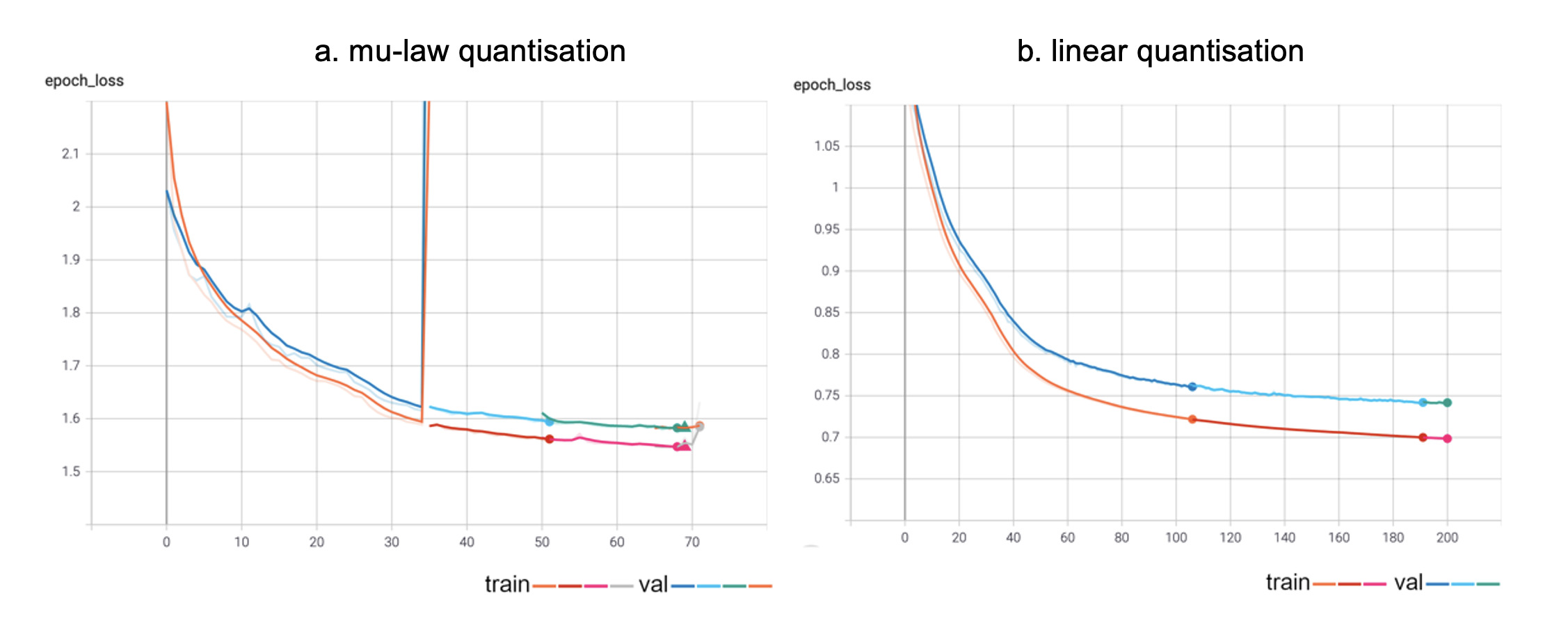
The screenshots below show graphs from TensorBoard³, TensorFlow’s tool for monitoring and visualising Machine Learning metrics and models.

Graphs from TensorBoard

More specifically, the graphs show the training and validation losses for the two training session, with each separate ‘run’ displayed in a separate colour (a ‘run’ is a single, uninterrupted sequence of training steps, usually over numerous epochs). The small circles indicate the ends of each run. The key at the bottom right of each graph shows the grouping of the lines under either the ‘training’ or ‘validation’. Notice that at one point in the first training session the gradient suddenly skyrockets, a phenomenon known as an ‘exploding gradient’. This can be caused by a number of things, the most common reason is when the model’s weights become very small, producing NaNs (‘Not a Number’). This is an uncommon experience when working with PRiSM SampleRNN – indeed this is only the second occasion it has occurred while training hundreds of models! The suggested solution is to lower the learning rate of the training – in this particular instance from 0.001 to 0.0001, which seemed to work, although the training did eventually grind to a halt. The graph from the linear quantised training is stable, however, which might be because the learning rate in that case was 0.0001 from the beginning.

In terms of the quality of the output (obviously I’m cherry-picking, it’s not all of this quality!), overall it’s pretty good, although the linear quantised training did produce some unpredictable, and annoying, bursts of noise. I think there is more than a hint of Beethoven in them, although my ear also detects some Schumann. And I also include one audio file (lvb_e=55_t=0.95_(9).wav) that, weirdly, sounds a lot like Stockhausen’s Mantra.

Notes

1. Before being fed to the model, samples from the dataset were quantized, which means converting the original samples, which might be floating point values, to an integer representation. Two quantization techniques were used, which not only display noticeable differences in the generated output, but also (as can be seen from the TensorBoard graphs) have an effect on training:

Mu-Law Quantization
This is a form of quantization which depends upon the fact that human hearing functions logarithmically. Sounds at higher levels do not require the same resolution as those at low levels, and mu-law quantization exploits this fact by ignoring the least significant bits in samples, compressing samples with 16 bits to 8 bits. The range of possible quantization levels in Mu-Law is therefore fixed at 0-255. Mu-Law is mainly used in North America, with the very similar A-Law quantization being popular in Europe.

Linear Quantization
With Linear Quantization we simply scale the input signal to a specific integer range (this may be 0-255, but can be larger or smaller). This type of quantization is agnostic with respect to the level of the signal, and treats all regions equally. Low-level parts of the signal are treated equally with high-level parts, which results in poor signal to noise ratios at lower levels. As is demonstrated by the generated examples, Mu-Law quantization offers somewhat better quality output, particularly at lower amplitudes. Linear quantization seemed did seem to offer better results when training, however, as the TensorBoard graphs show – the reason for this is still not clear, and is being investigated.

2 Epoch –  A single pass over the entire dataset during training. Temperature – A parameter used when generating output from a Machine Learning model which controls the amount of randomness in the output. The higher the temperature the more ‘surprising’ the generated samples.

3. TensorBoard is the tool bundled with TensorFlow for monitoring and visualising Machine Learning metrics and models, find out more about it here.